Análisis de regresión lineal múltiple

3.

El objetivo de los siguientes datos es analizar si el consumo de ciertos alimentos y otros factores (como edad, sexo, etc.) tienen una relación con el nivel de plasma beta-carotene. El interés original de estos datos fue recabar información que pudiera servir para encontrar los factores asociados con niveles bajos de plasma beta-carotene dado que estos podrían estar asociados con el riesgo de desarrollar algunos canceres.

Variables:

Dependiente. BETAPLASMA, Plasma beta-carotene (ng/ml)
Explicativas:
- AGE (years)
- SEX (1=Male, 2=Female)
- VITUSE, Vitamin Use (1=Yes, fairly often, 2=Yes, not often, 3=No)
- CALORIES, Number of calories consumed per day.
- FAT, Grams of fat consumed per day.
- FIBER, Grams of fiber consumed per day.
- ALCOHOL, Number of alcoholic drinks consumed per week.
- CHOLESTEROL, Cholesterol consumed (mg per day).
- BETADIET, Dietary beta-carotene consumed (mcg per day).

Datos=read.table("images/archivos/prdata.dat", 
           header=FALSE, sep="\t")
names(Datos)=c("AGE", "SEX", "SMOKSTAT", "QUETELET", "VITUSE", "CALORIES", "FAT", "FIBER", "ALCOHOL", "CHOLESTEROL", "BETADIET", "RETDIET", "BETAPLASMA", "RETPLASMA")

head(Datos)

str(Datos)

## 'data.frame':    315 obs. of  14 variables:
##  $ AGE        : int  64 76 38 40 72 40 65 58 35 55 ...
##  $ SEX        : int  2 2 2 2 2 2 2 2 2 2 ...
##  $ SMOKSTAT   : int  2 1 2 2 1 2 1 1 1 2 ...
##  $ QUETELET   : num  21.5 23.9 20 25.1 21 ...
##  $ VITUSE     : int  1 1 2 3 1 3 2 1 3 3 ...
##  $ CALORIES   : num  1299 1032 2372 2450 1952 ...
##  $ FAT        : num  57 50.1 83.6 97.5 82.6 56 52 63.4 57.8 39.6 ...
##  $ FIBER      : num  6.3 15.8 19.1 26.5 16.2 9.6 28.7 10.9 20.3 15.5 ...
##  $ ALCOHOL    : num  0 0 14.1 0.5 0 1.3 0 0 0.6 0 ...
##  $ CHOLESTEROL: num  170.3 75.8 257.9 332.6 170.8 ...
##  $ BETADIET   : int  1945 2653 6321 1061 2863 1729 5371 823 2895 3307 ...
##  $ RETDIET    : int  890 451 660 864 1209 1439 802 2571 944 493 ...
##  $ BETAPLASMA : int  200 124 328 153 92 148 258 64 218 81 ...
##  $ RETPLASMA  : int  915 727 721 615 799 654 834 825 517 562 ...

Usaremos, por simplicidad, variables binarias.

Datos$SEXFem=1*(Datos$SEX==2)
Datos$VITUSEYes=1*(Datos$VITUSE==1)
Datos$SEXFem=as.factor(Datos$SEXFem)
Datos$VITUSEYes=as.factor(Datos$VITUSEYes)

DatosRed=Datos[,c("BETAPLASMA", "AGE", "SEXFem", "VITUSEYes", "CALORIES", "FAT", "FIBER", "ALCOHOL", "CHOLESTEROL", "BETADIET", "VITUSE")]

summary(DatosRed)

##    BETAPLASMA        AGE     SEXFem  VITUSEYes    CALORIES         FAT     
##  Min.   :   0   Min.   :19   0: 42   0:193     Min.   : 445   Min.   : 14  
##  1st Qu.:  90   1st Qu.:39   1:273   1:122     1st Qu.:1338   1st Qu.: 54  
##  Median : 140   Median :48                     Median :1667   Median : 73  
##  Mean   : 190   Mean   :50                     Mean   :1797   Mean   : 77  
##  3rd Qu.: 230   3rd Qu.:62                     3rd Qu.:2100   3rd Qu.: 95  
##  Max.   :1415   Max.   :83                     Max.   :6662   Max.   :236  
##      FIBER       ALCOHOL     CHOLESTEROL     BETADIET        VITUSE    
##  Min.   : 3   Min.   :  0   Min.   : 38   Min.   : 214   Min.   :1.00  
##  1st Qu.: 9   1st Qu.:  0   1st Qu.:155   1st Qu.:1116   1st Qu.:1.00  
##  Median :12   Median :  0   Median :206   Median :1802   Median :2.00  
##  Mean   :13   Mean   :  3   Mean   :242   Mean   :2186   Mean   :1.97  
##  3rd Qu.:16   3rd Qu.:  3   3rd Qu.:309   3rd Qu.:2836   3rd Qu.:3.00  
##  Max.   :37   Max.   :203   Max.   :901   Max.   :9642   Max.   :3.00

library(GGally)
ggpairs(DatosRed[,c(1,3,4)])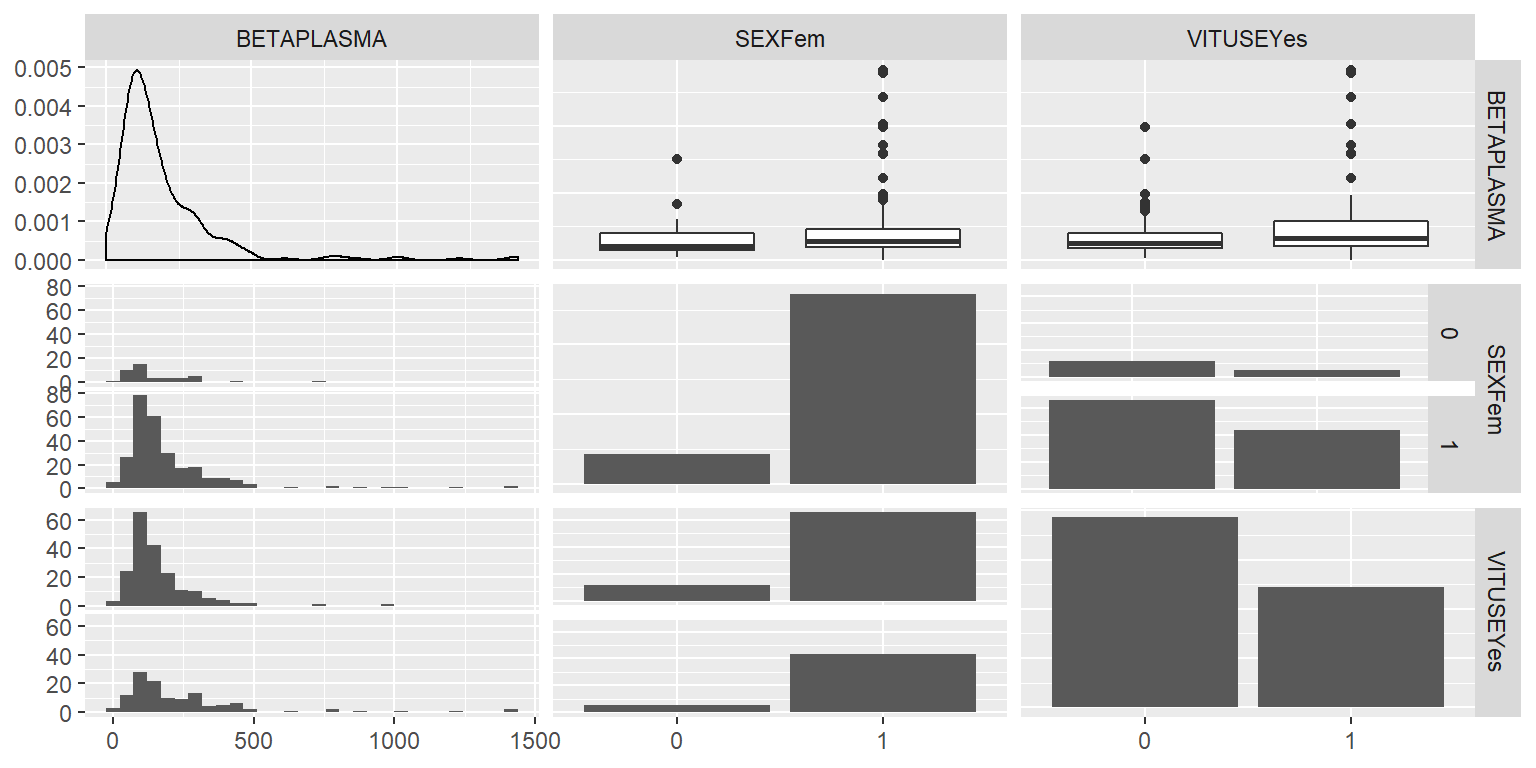

ggpairs(DatosRed[,c(1,2,5:10)])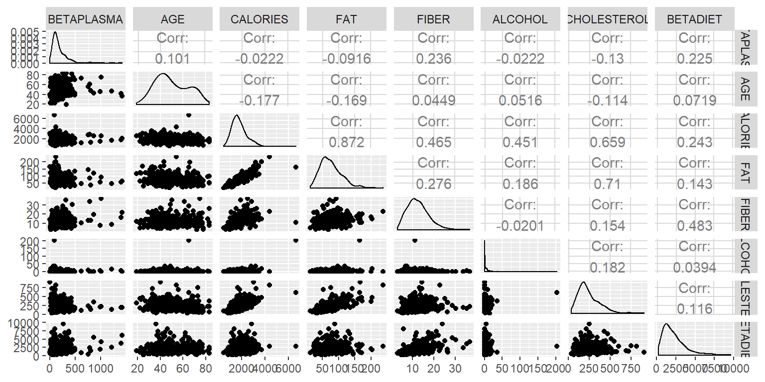

DatosRed[ DatosRed$ALCOHOL>100, ]

DatosRed[ DatosRed$CALORIES>4000, ]

DatosRed[ DatosRed$BETAPLASMA==0, ]

DatosRed2=DatosRed[-c(62, 257), ]

library(GGally)
ggpairs(DatosRed2[,c(1,3,4)])

ggpairs(DatosRed2[,c(1,2,5:10)])

DatosRed2$BETAPLASMAlog=log(DatosRed2$BETAPLASMA+10)


fit2=lm(BETAPLASMAlog~AGE+SEXFem+VITUSEYes+CALORIES+FAT+FIBER+ALCOHOL+CHOLESTEROL+BETADIET, data=DatosRed2)
summary(fit2)

## 
## Call:
## lm(formula = BETAPLASMAlog ~ AGE + SEXFem + VITUSEYes + CALORIES + 
##     FAT + FIBER + ALCOHOL + CHOLESTEROL + BETADIET, data = DatosRed2)
## 
## Residuals:
##     Min      1Q  Median      3Q     Max 
## -1.8298 -0.3546 -0.0217  0.3707  2.0218 
## 
## Coefficients:
##              Estimate Std. Error t value Pr(>|t|)    
## (Intercept)  4.27e+00   2.56e-01   16.69   <2e-16 ***
## AGE          5.05e-03   2.80e-03    1.81   0.0721 .  
## SEXFem1      2.80e-01   1.20e-01    2.33   0.0206 *  
## VITUSEYes1   2.24e-01   7.61e-02    2.94   0.0035 ** 
## CALORIES    -1.69e-04   1.92e-04   -0.88   0.3799    
## FAT          4.61e-04   3.03e-03    0.15   0.8792    
## FIBER        3.49e-02   1.06e-02    3.30   0.0011 ** 
## ALCOHOL      8.05e-03   8.21e-03    0.98   0.3277    
## CHOLESTEROL -4.18e-04   4.19e-04   -1.00   0.3193    
## BETADIET     4.19e-05   2.83e-05    1.48   0.1386    
## ---
## Signif. codes:  0 '***' 0.001 '**' 0.01 '*' 0.05 '.' 0.1 ' ' 1
## 
## Residual standard error: 0.64 on 303 degrees of freedom
## Multiple R-squared:  0.164,  Adjusted R-squared:  0.14 
## F-statistic: 6.62 on 9 and 303 DF,  p-value: 1.21e-08

drop1(fit2, test = "F")

Ejemplo con una variable categórica con 3 niveles.

DatosRed2$VITUSE=as.factor(DatosRed2$VITUSE)
fit3=lm(BETAPLASMAlog~AGE+SEXFem+VITUSE+CALORIES+FAT+FIBER+ALCOHOL+CHOLESTEROL+BETADIET, data=DatosRed2)
summary(fit3)

## 
## Call:
## lm(formula = BETAPLASMAlog ~ AGE + SEXFem + VITUSE + CALORIES + 
##     FAT + FIBER + ALCOHOL + CHOLESTEROL + BETADIET, data = DatosRed2)
## 
## Residuals:
##     Min      1Q  Median      3Q     Max 
## -1.9640 -0.3569 -0.0446  0.3606  1.8759 
## 
## Coefficients:
##              Estimate Std. Error t value Pr(>|t|)    
## (Intercept)  4.53e+00   2.64e-01   17.15  < 2e-16 ***
## AGE          5.55e-03   2.77e-03    2.00  0.04648 *  
## SEXFem1      2.37e-01   1.20e-01    1.98  0.04843 *  
## VITUSE2     -7.68e-02   9.18e-02   -0.84  0.40324    
## VITUSE3     -3.42e-01   8.63e-02   -3.96  9.3e-05 ***
## CALORIES    -2.32e-04   1.91e-04   -1.21  0.22671    
## FAT          1.47e-03   3.02e-03    0.49  0.62706    
## FIBER        3.61e-02   1.04e-02    3.46  0.00062 ***
## ALCOHOL      9.85e-03   8.15e-03    1.21  0.22726    
## CHOLESTEROL -4.40e-04   4.14e-04   -1.06  0.28903    
## BETADIET     4.06e-05   2.79e-05    1.45  0.14761    
## ---
## Signif. codes:  0 '***' 0.001 '**' 0.01 '*' 0.05 '.' 0.1 ' ' 1
## 
## Residual standard error: 0.63 on 302 degrees of freedom
## Multiple R-squared:  0.185,  Adjusted R-squared:  0.158 
## F-statistic: 6.88 on 10 and 302 DF,  p-value: 1.09e-09

drop1(fit3, test = "F")

Para la variable VITUSE

library(multcomp)
K=matrix(c(0,0,0,1,0,0,0,0,0,0,0, 0,0,0,0,1,0,0,0,0,0,0), ncol=11, nrow=2, byrow=TRUE)
m=c(0, 0)
summary(glht(fit3, linfct=K, rhs=m),test=Ftest())

## 
##   General Linear Hypotheses
## 
## Linear Hypotheses:
##        Estimate
## 1 == 0  -0.0768
## 2 == 0  -0.3419
## 
## Global Test:
##      F DF1 DF2 Pr(>F)
## 1 8.33   2 302  3e-04

Para categorías de la variable VITUSE

library(multcomp)
K=matrix(c(0,0,0,1,-1,0,0,0,0,0,0), ncol=11, nrow=1, byrow=TRUE)
m=c(0)
summary(glht(fit3, linfct=K, rhs=m),test=Ftest())

## 
##   General Linear Hypotheses
## 
## Linear Hypotheses:
##        Estimate
## 1 == 0    0.265
## 
## Global Test:
##      F DF1 DF2  Pr(>F)
## 1 7.83   1 302 0.00547

Análisis de regresión lineal múltiple

Gonzalo Pérez

13 de abril de 2020

3.